
Sometimes easy concepts are made so easy you can get confused.
I’m reading a book titled Statistical Rethinking: a bayesian course with examples in R and Stan, written by Richard McElreath.
I really appreciate this book. I feel like the way that I was taught statistics in psychology really missed the mark. I like how the author in this book frames the differences between bayesian in frequentist statisticians, basically reducing them to their goals.
I’m having to read slowly–mostly because we have a newborn in the house and I’m very much sleep derived. But I also want to make sure that I understand what I’m reading and I think the author did a very good job of setting up the purpose of grid approximation, it’s just that for some reason I had a hard time understanding what the they were for.
It’s basically a way to start generating, what’s known in Bayesian inference, a prior.
But even that is mysterious. Let’s say you have some method for making predictions. This method takes several variables to work. If you know the values for these variables you can use your method and make your prediction.
Well, what if you don’t know all the variables? You’ll need to estimate one or several. And the prior is what begins this process.
After you’ve completed a Bayesian analysis, the output will be a distribution of values for that unknown variable. This distribution will give you some ability to quantify your belief in that value.
A Bayesian model is going to mechanically churn out a probability for the phenomenon but before it does that it needs a starting condition, and this is the prior.
The book offers a few ways to obtain a prior, and the author begins with grid_approximation.
In my own words, it’s like taking a prior probability but then spreading it across a range. This range is then fed into the Bayesian model.
In other words, if you think the prior is a 50/50 situation, that each outcome is equally likely, you can spread that assumption across a grid and let the model try on the range of scores.
The book has a thought experiment trying to estimate water coverage over a hypothetical globe. Let’s say the data is 6 w in 9 observations.
This set up fits nicely to a binomial distribution, but what are the parameters? Should Pr(water) =0.5?
Doing this you’d calculate a Bayesian posterior of
dbinom(6,9,.5)
[1] 0.1640625
But if you took that 0.5 and spread it across a range from 0 to 1, you’d get a distribution of scores, and with a distribution you have more options to study the effectiveness of your model.
Just spreading out that .5 belief into 5 different values from 0 to 1 we get this data.frame, where the first column represents a prior whole the second column is the posterior estimate for the prior:
p_grid posterior
[1,] 0.00 0.00000000
[2,] 0.25 0.02129338
[3,] 0.50 0.40378549
[4,] 0.75 0.57492114
[5,] 1.00 0.00000000
Dbinom(6,9,.75):
[1] 0.2335968
So, a better estimate.
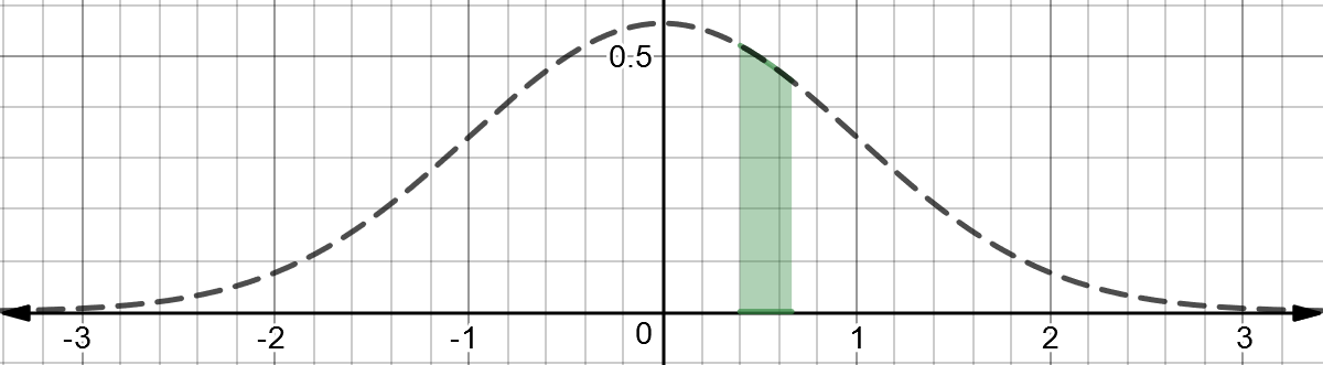
Spreading the prior across 50 intervals gets you a distribution like this:

The posterior score in the y axis will continue to shrink as the x axis goes to infinity–this is a property of probability distributions. The probability of a function is basically the area under the curve and since a single point can not have area under it, just a line, it’s probability is zero. Of course we can take a range.
Anyway, trying to wrap my head around priors and their estimates. The distribution above, a posterior distribution, is simply a distribution of possible values for a variable in the model. This variable is called a parameter and it is what we are trying to estimate.
